Deep Learning Engineering Tricks

Deep learning is full of little engineering tricks (that are sometimes omitted from the papers!), and these are responsible for getting those last few points that will get you state of the art. Here, we go through them one by one, giving an explanation as to how and why they work alongside an intuition as to where they should be used.

Initialisation

Weight initialisation is done during the __init__ portion of a model and involves setting the starting weights of the various module components. If your model has good weight initialisation, then the less work the first few training epochs have to do in order to get your model to learn a good approximation. Get this right and the model will have to spend less time learning the basics of your data.

Initialisation of weights can be: random, constant, sampled from a uniform distribution, or sampled from a normal distribution. Depending on the weights being initialised, a different approach is needed. Something else that will impact the type of weight initialisation that is used is the activation function. For example, you won’t want a constant initialisation of 0 before a ReLU activation.

Xavier Initialisation

The Xavier initialisation method was designed specifically for use with the sigmoid and tanh activation functions. The curve of these functions is such that the central part is almost linear and the extremes have an output that tends to 0 as the curve flattens more. This means the activation function is most effective when the values fall where the gradient is highest.

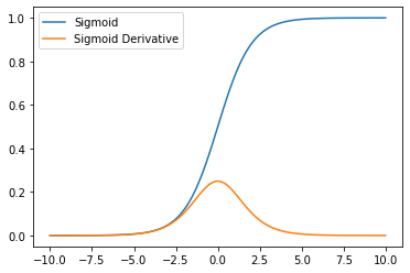
We therefore want to initialise the network weights in such a way that they interact with the input data to produce an output that falls within the effective range of the activation function. Notice how the gradient of the sigmoid function looks like a normal distribution? We therefore want to initialise network weights to produce outputs that fall nicely within the derivative of the sigmoid.

Given a random input and a weight matrix that has been random initialisation, we can visualise the output of computing the forward pass of a linear layer before it is passed to the activation function (on the left) as well as after the sigmoid function (on the right).

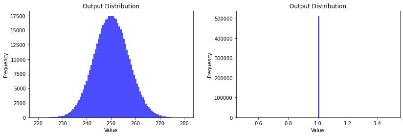
As we can see, the output values centre around 250, which results in the sigmoid becoming saturated at 1. By introducing the Xavier initialisation, we can resolve this issue.

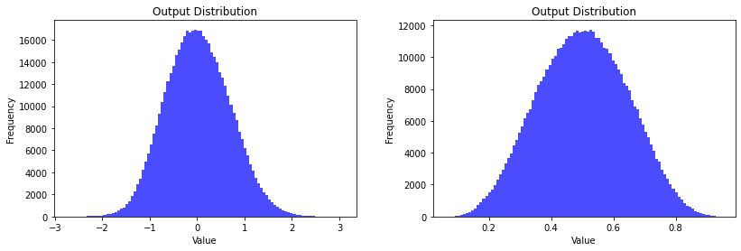
Notice how prior to the activation function, the output distribution (left) is centred around 0. This enables to sigmoid to have a better range of activations. As a result, the network can more easily shift the distributions to learn the patterns of the data.

Kaiming Initialisation

The Kaiming initialisation strategy addresses shortcomings that the Xavier approach has when used with the ReLU family of activation functions. It works by increasing the variance of the normal distribution used to initialise the weights, which in turn increases the chance of the output neuron being greater than 0 (and therefore activating in ReLU).

[!WARNING] Bias Terms Remember to initialise the bias terms (if used) to 0 when using Kaiming intialisation

Orthogonal Initialisation

A matrix \(\mathbf{W}\) is orthogonal if \(\mathbf{W}^\top\mathbf{W} = \mathbf{I}\). Orthogonal initialisation is a technique creating weight matrices that are orthogonal. By initialising the weights in such as way, we can ensure that the norm (length) of any input vector is preserved in the output vector. In other words, if the weight matrix \(\mathbf{W}\) processes the input vector \(\mathbf{x}\) to give the output vector \(\mathbf{y}\) i.e. \(\mathbf{y} = \mathbf{Wx}\), then \(\|\mathbf{x}\| = \|\mathbf{y}\|\). By preserving the norm of the input vector, it can prevent the values of the vector increasing or decreasing too rapidly, in turn preventing the exploding and vanishing gradient problems. Stabilising the gradients of the weight matrices in such a way ensures that the optimisation process stays within a more reasonable window of parameters, leading to faster convergence.

Orthogonal initialisation is therefore most beneficial where exploding/vanishing gradients are a problem or where large matrices are used. This makes them particularly useful in RNNs and CNNs.

A Note for PyTorch Users

[!Warning] Remember the gain Depending on the gain of the activation function, the initialisation can be different. By default, the initialisation functions use a gain=1.0. However, in Xavier and Kaiming initialisation you should pass in gain=nn.init.calculate_grain('<ACTIVATION FUNCTION NAME>')

Regularisation

Regularisation is a set of techniques used to prevent overfitting, or put differently, to improve the generalisability of the model.

Dropout

Dropout is useful to avoid overfitting when working with small data sets. Based on this paper by Hinton et al., it will randomly (via Bernoulli distribution) zero some elements of the input tensor. In other words, \(p\%\) of elements in the input tensor will be zeroed. The intuition is to add some noise to the signal produced by neurons in the network to prevent overfitting.

Outputs are also scaled by a factor of \(\frac{1}{1-p}\) during training. \(p=0\) at evaluation time.

From the little book of Deep Learning pg 72:

The motivation behind dropout is to favour meaningful individual activation and discourage group representation. Since the probability that a group of $k$ activations remain intact through the dropout layer is $(1-p)^k$, joint representations become unreliable, making the training procedure avoid them. It can also be seen as noise injection that makes the training more robust.

[!INFORMATION] Setting p For intermediate layers, choosing (1-p) = 0.5 for large networks is ideal. For the input layer, (1-p) should be kept about 0.2 or lower. This is because dropping the input data can adversely affect the training. A (1-p) > 0.5 is not advised, as it culls more connections without boosting the regularization. Source

Dropout should be used on the layers that are prone to overfitting, which are typically the deeper layers within a network.

L1 (Laso) Regularisation

In L1 regularisation, a penalty term is added to the loss function to introduce sparsity (setting weights to 0) in the model. The penalty term is the sum of the absolute values of the weights, scaled by a hyperparameter \(\lambda\). Introducing the L1 regularisation penalty to the loss function encourages the model to push certain weights to $0$. Through introducing more sparsity, the model is effectively selecting a subset of the input features which it deems to be the most important. In other words, it can be viewed as a type of built in feature selection.

L2 (Ridge) Regularisation

This is implemented as part of the PyTorch optimiser through the weight_decay parameter. Note that it is set to 0 in Adam and 0.01 in AdamW. It works by adding the sum of the squares of all the model weights (multiplied by a parameter \(\lambda\)) to the loss. L2 regularisation works as a penalty (adding it makes the loss higher), and forces the model to learn smaller weights. The model should become more generalisable when learning smaller weights as it becomes less sensitive to particular inputs. When models have uneven weight distributions, where certain weights dominate over others in the layer, they essentially end up “memorising” the training data.

Normalisation

Remember back to the initialisation stage of the neural network, where it was beneficial for the weight distribution to roughly follow a Gaussian distribution. It turns out that maintaining this distribution later on in the network is also beneficial as it prevents layers being dominated by a few parameters. Normalisation layers tweak the distribution of the weight parameters in the network to nudge them back towards a more Gaussian distribution. However, we don’t want to force a pure (unit) Gaussian distribution, rather, we want to let the network decide what the shape of the Gaussian looks like. To achieve this, normalisation layers include a scale and shift operation alongside the normalisation.

It is typical to place normalisation layers after layers that contain multiplication (linear layers, convolutional layers etc) and before any non-linearity.

Batch Normalisation

Batch normalisation as a regulariser: One of the downsides of batch normalisation is that it couples all the elements of a batch together. Rather than have all the elements in a batch be independent, the elements are normalised according to the other elements in the batch - therefore coupling them all together. This means the normalisation is dependent on the randomly sampled batch elements, which introduces a certain amount of noise into training. Which, from dropout we know to be a benefit in training.

[!TIP] Layer Biases If the layer before the batch normalisation has a bias term, it will essentially be removed by the batch normalisation layer. Therefore, it is best to pass bias=False into the network layer.

Batch normalisation presents a distinct challenge: it forces batches into the architecture of the network, so what happens when the batch size is $1$? To alleviate this, at inference the normalisation uses statistics calculated over the entire training set. However, this would involve us having to compute these statistics in addition to the train and test loops. So, to avoid this, an estimation of the mean and standard deviation of the whole training set is calculated throughout the training for use during inference. \(\hat{x}_i = \frac{x_i - \mu_B}{\sqrt{\sigma_B^2 + \epsilon}}\) Where:

• \(x_i\) is the i-th input feature
• \(\mu_B\) is the mean of the batch
• \(\sigma_B^2\) is the variance of the batch
• \(\epsilon\) is a small constant added for numerical stability

The batch normalisation layer applies this transformation to each input feature, normalising the inputs to have zero mean and unit variance within each batch.

Layer Normalisation

Layer normalisation is very similar to batch normalisation. But, instead of normalising across the batch dimension, it normalises against the layer dimension. This makes it effective for sequence modelling or when the batch dimension is small or variable. \(\hat{x}_i = \frac{x_i - \mu_L}{\sqrt{\sigma_L^2 + \epsilon}}\) Where:

• \(x_i\) is the i-th input feature
• \(\mu_L\) is the mean of all the features in the same layer
• \(\sigma_L^2\) is the variance of all the features in the same layer
• \(\epsilon\) is a small constant added for numerical stability

The key difference between batch normalisation and layer normalisation is that layer normalisation computes the mean and variance across all the features in the same layer, rather than across the batch dimension. This makes layer normalisation independent of the batch size and more suitable for tasks with variable batch sizes or sequential data.

Root Mean Square Layer Normalisation

RMSNorm is a simplification of the Layer Normalisation technique that reduces the computation overhead through the removal of the mean centring operation. \(\hat{x}_i = \frac{x_i}{\sqrt{\frac{1}{d}\sum_{j=1}^{d}x_j^2 + \epsilon}}\) Where:

• \(x_i\) is the i-th input feature
• \(d\) is the number of features in the input
• \(\epsilon\) is a small constant added for numerical stability

RMSNorm is a variant of layer normalisation that uses the root mean square (RMS) of the input features instead of the standard deviation. The RMS is calculated across all the features in the same layer, similar to layer normalisation.

The key difference is that RMSNorm does not subtract the mean from the input features before normalisation, but instead divides the input features by their RMS. This can provide better performance in some cases, especially for tasks where the mean of the input features is not informative.