Hello World - Deep Learning Style: PyTorch and MNIST
In this tutorial you will set up a clean Python environment, install PyTorch, and train a neural network to recognise handwritten digits from the MNIST dataset - the “hello world” of deep learning. Everything is explained as we go; no prior machine learning knowledge is assumed, only basic Python.
What you’ll end up with: a model that looks at a 28×28 greyscale image of a handwritten digit and tells you which digit (0–9) it is, with ~98% accuracy, trained in a couple of minutes on your CPU.
1. The big picture
Before touching any code, it helps to know what “training” actually means.
A neural network is a function with millions (billions, or even trillions!) of adjustable dials called weights. Initially the dials are set to random values, so the function outputs garbage. Training is an automatic dial-adjusting procedure:
- Show the network an input (in this case, an image - e.g. a handwritten “7”).
- It makes a guess (probably wrong at first - it’s random).
- A loss function measures how wrong the guess was, as a single number.
- Backpropagation works out which way to turn each dial to make the loss slightly smaller (this is just the chain rule from calculus, applied a million times).
- An optimiser nudges every dial a tiny step in that direction. The step size is called the learning rate.
- Repeat with thousands of images. The loss drops, the guesses (hopefully) get good.
2. Setup: Python, venv, and PyTorch
Create and activate the venv
You need Python 3.9 or newer (python3 --version to check). Then, in a fresh project folder:
# Create the environment (a folder called .venv)
python3 -m venv .venv

# Activate it - macOS/Linux:
source .venv/bin/activate

# Activate it - Windows (Command Prompt):
.venv\Scripts\activate.bat
# or Windows (PowerShell):
.venv\Scripts\Activate.ps1
Your shell prompt should now start with (.venv). From now on, python and pip refer to the isolated copies. To leave the environment later, run deactivate. To come back, source .venv/bin/activate again.
Install PyTorch
pip install torch torchvision matplotlib
- torch - the core PyTorch library: tensors (multi-dimensional arrays) plus the automatic differentiation engine that does backpropagation for us.
- torchvision - companion library with ready-made datasets (including MNIST) and image utilities.
- matplotlib - for plotting a few images so we can see the data.
Note: this installs the CPU version of PyTorch, which is all you need here - MNIST is tiny. If you later work on bigger models with an NVIDIA GPU, you’d install a CUDA-enabled build from pytorch.org.
Sanity check:
python -c "import torch; print(torch.__version__)"
If a version number prints, you’re set.
3. The code, piece by piece
Create a file called train_mnist.py. We’ll build it up in sections, and the full listing is at the end. (Or: read the explanations, then just run the full listing.)
3.1 The data
from torchvision import datasets, transforms
from torch.utils.data import DataLoader

transform = transforms.ToTensor()

train_data = datasets.MNIST(root="data", train=True,  download=True, transform=transform)
test_data  = datasets.MNIST(root="data", train=False, download=True, transform=transform)

train_loader = DataLoader(train_data, batch_size=64, shuffle=True)
test_loader  = DataLoader(test_data,  batch_size=1000)
- MNIST is 70,000 greyscale images of handwritten digits: 60,000 for training, 10,000 held back for testing.
download=Truefetches it on first run. - Keeping a test set the model never trains on is essential: it’s how we measure whether the model learned general patterns rather than memorising its homework.
transforms.ToTensor()converts each image from a PIL image (pixels 0–255) into a PyTorch tensor of shape[1, 28, 28]with values scaled to 0.0–1.0. Neural nets want numbers, not image files.- A DataLoader feeds data to the model in batches of 64 images rather than one at a time. Batching is much faster (matrix operations love bulk) and makes training less noisy.
shuffle=Truerandomises the order each pass so the model doesn’t learn anything spurious from the ordering.
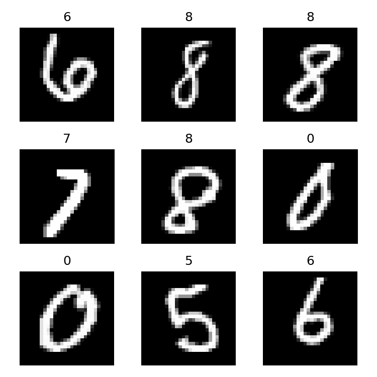
Want to see the data? This snippet saves a plot of the first 9 examples:
import matplotlib.pyplot as plt

images, labels = next(iter(train_loader))
fig, axes = plt.subplots(3, 3)
for ax, img, label in zip(axes.flat, images, labels):
    ax.imshow(img.squeeze(), cmap="gray")
    ax.set_title(label.item()); ax.axis("off")
plt.savefig("mnist_examples.png")
3.2 The model
import torch.nn as nn

model = nn.Sequential(
    nn.Flatten(),          # [1, 28, 28] -> [784]
    nn.Linear(784, 128),   # fully-connected layer
    nn.ReLU(),             # non-linearity
    nn.Linear(128, 10),    # one output score per digit 0-9
)
This is a small fully-connected (a.k.a. MLP) network:
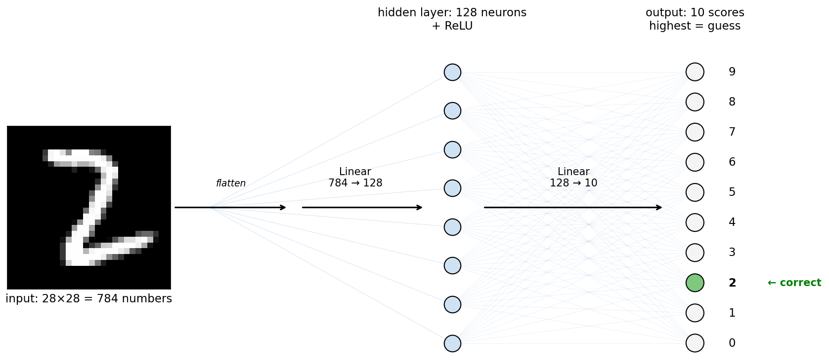
nn.Flatten()- an image is a 28×28 grid, but a plain linear layer wants a flat vector, so we unroll it into 784 numbers.nn.Linear(784, 128)- a classic matrix multiply plus bias:y = Wx + b. It has 784×128 + 128 = 100,480 weights. These are the “dials”. Each of the 128 outputs can learn to detect some pattern in the pixels.nn.ReLU()- sets negative values to zero (max(0, x)). Without a non-linearity between layers, stacking linear layers is pointless - two matrix multiplies in a row collapse into one. ReLU is what lets the network learn curved, complicated decision boundaries.nn.Linear(128, 10)- maps down to 10 raw scores (logits), one per digit. The highest score is the model’s guess. (Use a softmax function to turn logits into probabilities).
3.3 Loss and optimiser
loss_fn = nn.CrossEntropyLoss()
optimiser = torch.optim.SGD(model.parameters(), lr=0.05, momentum=0.9)
CrossEntropyLossturns the 10 logits into probabilities and penalises the model based on how little probability it gave the correct digit. Confident and wrong → big loss. Confident and right → tiny loss.SGD(stochastic gradient descent) is the optimiser - the dial-nudging step from section 1 made literal. Each weight moves a small step opposite its gradient, scaled by the learning rate (lr=0.05). “Stochastic” because each step uses a random batch of 64 images, not the whole dataset.momentum=0.9- each update keeps 90% of the previous update’s direction, like a ball rolling downhill: it smooths out zigzagging and builds up speed along consistent slopes, so SGD converges much faster. These two values (lr=0.05,momentum=0.9) are standard starting points.
Watch out for the learning rate in the exercises below: too high and training oscillates or explodes; too low and it crawls. There’s a popular, more forgiving alternative to SGD called Adam - exercise 6 has you compare them.
3.4 The training loop
This is the heart of it - five lines that are the same in nearly every PyTorch project you’ll ever see:
for epoch in range(5):                     # 5 passes over the whole dataset
    for images, labels in train_loader:    # 64 images at a time
        optimiser.zero_grad()              # 1. clear old gradients
        logits = model(images)             # 2. forward pass
        loss = loss_fn(logits, labels)     # 3. how wrong were we?
        loss.backward()                    # 4. compute gradients
        optimiser.step()                   # 5. nudge the weights
    print(f"epoch {epoch+1} done, last batch loss: {loss.item():.4f}")
One pass through all 60,000 images is an epoch. Step 4 is where PyTorch earns its keep: loss.backward() automatically computes the gradient of the loss with respect to every single weight - no manual calculus required. Step 5 uses those gradients to update the weights.
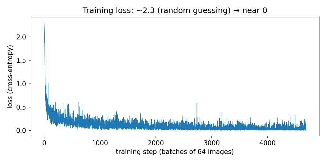
Watch the printed loss: it should fall from ~2.3 (random guessing: ln(10) ≈ 2.3) to well under 0.1. That number going down is learning.
3.5 Did it actually learn? Evaluation
model.eval()  # tell the model we're testing, not training

correct = 0
with torch.no_grad():                      # don't track gradients here
    for images, labels in test_loader:
        predictions = model(images).argmax(dim=1)  # index of max score
        correct += (predictions == labels).sum().item()

print(f"Test accuracy: {correct / len(test_data):.1%}")
We run the model over the 10,000 images it has never seen, take the highest-scoring digit as its prediction (argmax), and count correct answers. torch.no_grad() disables the gradient bookkeeping, saving time and memory. Expect ~97–98%.
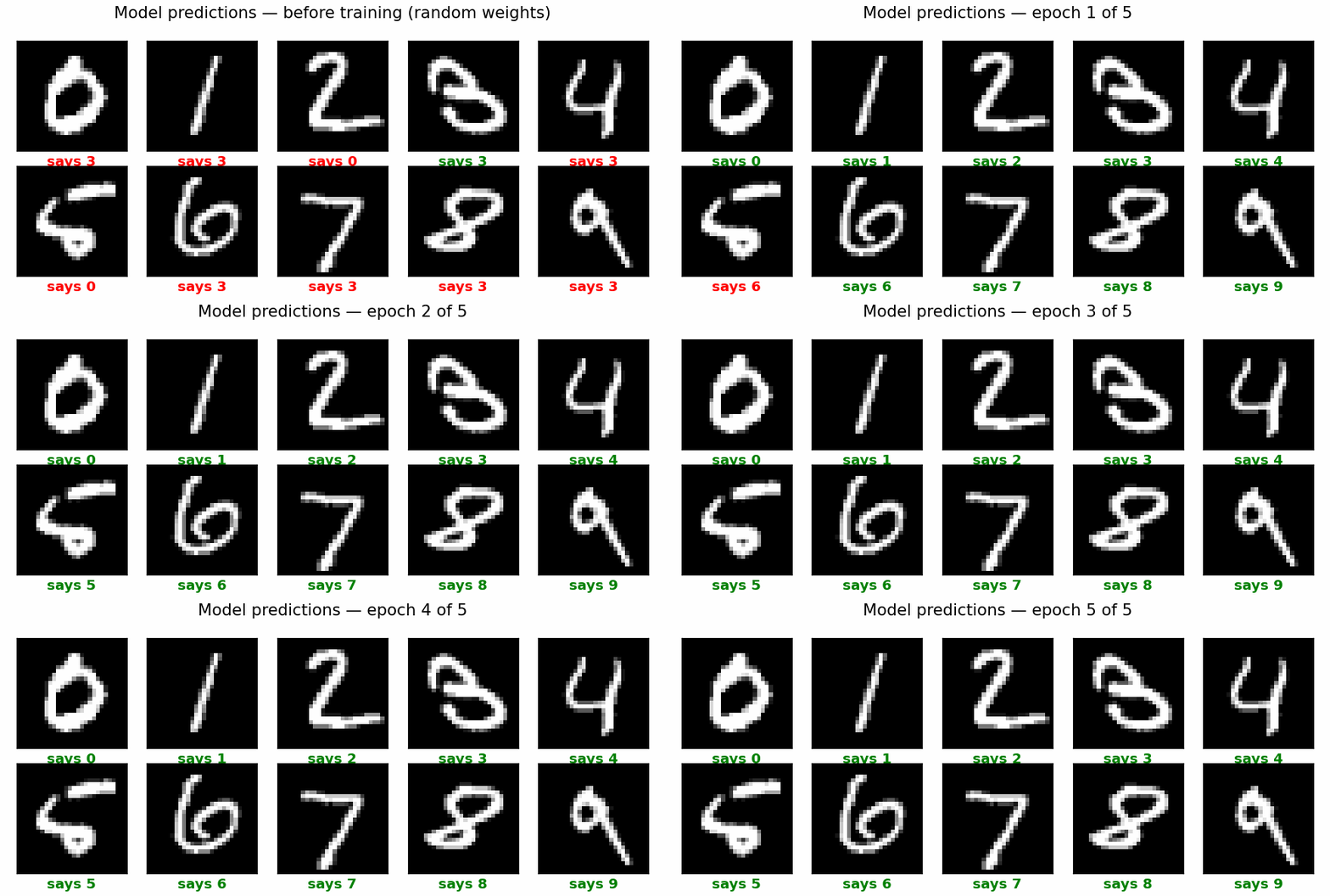
Here is the same model, frame by frame, learning to classify ten test digits it never trained on (green = correct, red = wrong):
4. Run it
python train_mnist.py
First run downloads MNIST (~10 MB) into data/, then trains for 5 epochs - a couple of minutes on a laptop CPU.
5. Full listing
import torch
import torch.nn as nn
from torchvision import datasets, transforms
from torch.utils.data import DataLoader

# --- Data ---
transform = transforms.ToTensor()
train_data = datasets.MNIST(root="data", train=True,  download=True, transform=transform)
test_data  = datasets.MNIST(root="data", train=False, download=True, transform=transform)
train_loader = DataLoader(train_data, batch_size=64, shuffle=True)
test_loader  = DataLoader(test_data,  batch_size=1000)

# --- Model ---
model = nn.Sequential(
    nn.Flatten(),
    nn.Linear(784, 128),
    nn.ReLU(),
    nn.Linear(128, 10),
)

loss_fn = nn.CrossEntropyLoss()
optimiser = torch.optim.SGD(model.parameters(), lr=0.05, momentum=0.9)

# --- Train ---
for epoch in range(5):
    for images, labels in train_loader:
        optimiser.zero_grad()
        logits = model(images)
        loss = loss_fn(logits, labels)
        loss.backward()
        optimiser.step()
    print(f"epoch {epoch+1} done, last batch loss: {loss.item():.4f}")

# --- Evaluate ---
model.eval()
correct = 0
with torch.no_grad():
    for images, labels in test_loader:
        predictions = model(images).argmax(dim=1)
        correct += (predictions == labels).sum().item()
print(f"Test accuracy: {correct / len(test_data):.1%}")

# --- Save ---
torch.save(model.state_dict(), "mnist_model.pt")
The last line saves the trained weights to mnist_model.pt, so you can reload them later (model.load_state_dict(torch.load("mnist_model.pt"))) without retraining.
6. Things to try
The fastest way to build intuition is to break things on purpose:
- Remove the ReLU. What happens to accuracy? Why?
- Change the learning rate to
1e-1, then1e-5. What changes? - Make the hidden layer bigger (128 → 512) or add another
Linear/ReLUpair. Does it help? - Train for 1 epoch instead of 5. Where’s the trade-off?
- Look at its mistakes: collect test images where the model was wrong and plot them. Would you have got them right?
- Switch optimisers. Replace the SGD line with
torch.optim.Adam(model.parameters(), lr=1e-3)and rerun, noting test accuracy after each epoch. Adam adapts the step size for every weight individually, so it works well with almost no tuning - expect ~94% after one epoch, ~97% after five. But compare honestly with what you just got from tuned SGD (~96% after one, ~98% after five): on this simple problem SGD actually edges it out. The real lesson: Adam’s advantage is needing less tuning, which is why it’s the modern default - not that it’s magically better. On big models with messy loss surfaces, that tuning-free robustness matters much more than it does here.
7. Where next?
- This model ignores the spatial structure of images (it flattens them). Convolutional networks (
nn.Conv2d) exploit that structure - see the extension in section 8 below. - The official PyTorch tutorials at pytorch.org/tutorials pick up exactly where this leaves off.
8. Extension: a convolutional network (LeNet)
Our MLP flattens each image into 784 unrelated numbers - it has no idea that two neighbouring pixels form an edge, or that a “7” is a “7” whether it’s centred or shifted two pixels left. A convolutional neural network (CNN) builds that knowledge in.
LeNet-5 (LeCun et al., 1998) is the original CNN, designed for exactly this digit-recognition task. It introduces two layer types:
nn.Conv2d- instead of connecting every pixel to every neuron, a small kernel (here 5×5) slides across the image, detecting the same pattern everywhere: a horizontal edge is a horizontal edge wherever it appears. Each kernel produces a feature map highlighting where its pattern occurs. The first conv learns 6 such detectors, the second 16 (looking for combinations of the first layer’s edges - curves, corners, loops).nn.MaxPool2d(2)- shrinks each feature map by taking the max of every 2×2 block. This halves the resolution (cheap) and makes detection slightly tolerant to small shifts: roughly where the edge was matters less than that it was found.
lenet = nn.Sequential(
    nn.Conv2d(1, 6, kernel_size=5), nn.ReLU(), nn.MaxPool2d(2),   # 28→24→12
    nn.Conv2d(6, 16, kernel_size=5), nn.ReLU(), nn.MaxPool2d(2),  # 12→8→4
    nn.Flatten(),
    nn.Linear(16 * 4 * 4, 120), nn.ReLU(),
    nn.Linear(120, 84), nn.ReLU(),
    nn.Linear(84, 10),
)
Note the shape bookkeeping in the comments: a 5×5 kernel on a 28×28 image produces 24×24 (it can’t centre on the outer 2 pixels), then pooling halves it to 12×12, and so on - ending with 16 maps of 4×4, flattened to 256 numbers for the classifier part. Everything else - data, loss, optimiser, training loop - is identical to before. Swap the model definition and rerun.
Does it help?
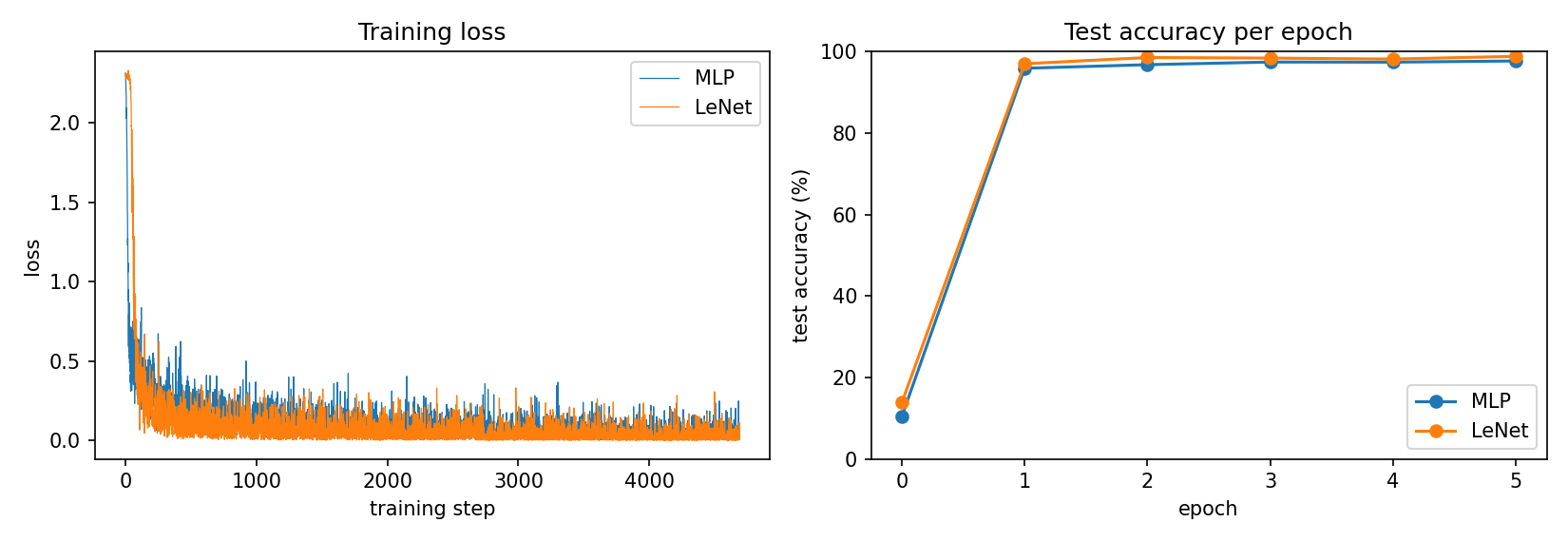
Both models trained for 5 epochs, same settings, on the same machine:
| Model | Test accuracy | Parameters | Training time (CPU) |
|---|---|---|---|
| MLP | 97.8% | 101,770 | ~6 s |
| LeNet | 98.9% | 44,426 | ~28 s |
Three takeaways:
- LeNet is more accurate with less than half the parameters. Exploiting image structure means it needs fewer dials to do a better job - weight sharing (one kernel reused everywhere) is very parameter-efficient.
- It’s slower per step. Convolutions are more arithmetic than a matrix multiply, and on a CPU you feel it. (On a GPU this gap shrinks dramatically - convolutions parallelise beautifully.)
- The gap looks small because MNIST is easy. 97.8% vs 98.9% is ~110 fewer misclassified digits out of 10,000 - meaningful, but not dramatic. On harder, real-world images the MLP plateaus quickly while CNNs keep climbing; that difference is why CNNs took over computer vision.
To see its mistakes for yourself, reuse exercise 5 from section 6 with lenet - you’ll find the remaining errors are mostly digits even humans would squint at.
9. Extension: standing on giants’ shoulders — fine-tuning a pretrained ResNet
So far we’ve trained every weight from random initialisation. In practice, nobody does this unless they have to: you download a network someone else trained for weeks on a giant dataset, and fine-tune it for your problem. This is called transfer learning, and it’s how most real-world deep learning gets done.
ResNet and residual connections, in one paragraph
ResNet (He et al., 2015) is the architecture that made very deep networks trainable. Stacking more layers should help, but past a certain depth training got worse — gradients degrading as they pass through dozens of layers. ResNet’s fix is the residual (skip) connection: each block computes output = F(x) + x — the layer learns only a correction to its input rather than a whole new transformation, and gradients can flow backwards through the + x shortcut untouched. That one trick enabled networks 100+ layers deep and won the ImageNet competition in 2015. We’ll use ResNet-18 (18 layers, ~11 million parameters) — small by modern standards, huge next to our LeNet.
The fine-tuning recipe
Step 1 — load it pretrained. weights="DEFAULT" downloads weights trained on ImageNet: 1.2 million photographs across 1,000 classes. Its early layers already detect edges, textures and shapes — features any vision task can reuse.
from torchvision import models

model = models.resnet18(weights="DEFAULT")   # ~45 MB download, once
Step 2 — replace the head. The last layer outputs 1,000 ImageNet class scores. We don’t care about those classes — chop it off and attach a fresh, randomly-initialised layer for our 10 digits:
model.fc = nn.Linear(model.fc.in_features, 10)
Step 3 — adapt the inputs. The pretrained network expects 3-channel images, roughly photo-sized, scaled the way ImageNet images were scaled (these magic numbers are ImageNet’s channel means and standard deviations):
transform = transforms.Compose([
    transforms.Resize(64),        # 28×28 is tiny for a deep network
    transforms.Grayscale(3),      # copy the one channel into three
    transforms.ToTensor(),
    transforms.Normalize(mean=[0.485, 0.456, 0.406],
                         std=[0.229, 0.224, 0.225]),
])
Step 4 — train the head only (backbone frozen). Freezing means requires_grad = False: no gradients, no updates — the pretrained features stay put, and only our 5,130 new head weights learn. This is fast and safe.
for p in model.parameters():
    p.requires_grad = False          # freeze the backbone
for p in model.fc.parameters():
    p.requires_grad = True           # ...except the new head

optimiser = torch.optim.SGD(model.fc.parameters(), lr=0.05, momentum=0.9)
# ... same training loop as before ...
Step 5 — unfreeze and fine-tune gently. Now let the whole network adjust, but with a much smaller learning rate (0.005, not 0.05): the pretrained weights are already good, and big steps would wreck them. One epoch is enough to see the effect.
for p in model.parameters():
    p.requires_grad = True
optimiser = torch.optim.SGD(model.parameters(), lr=0.005, momentum=0.9)
# ... same training loop again ...
What actually happens
Run on a 12,000-image training subset (to keep CPU time in minutes rather than hours), test accuracy after each stage:
| Model | Test accuracy | Parameters | Cost |
|---|---|---|---|
| MLP (§3) | 97.8% | 101,770 | ~6 s total |
| LeNet (§8) | 98.9% | 44,426 | ~28 s total |
| ResNet-18, head only (frozen) | 82.7% | 11.2M (5,130 trained) | ~50 s/epoch |
| ResNet-18, fully fine-tuned (1 epoch) | 97.7% | 11.2M | ~18 min |
Three lessons, and the first one surprises most people:
- Pretrained ≠ instantly good. With the backbone frozen, accuracy stalls around 80% — worse than our MLP. ImageNet is photographs of objects; MNIST is white pen strokes on black. The pretrained features detect fur, wheels and textures — not strokes. Transfer works best when the original and new tasks are similar; here the domain gap is real.
- Unfreezing closes the gap fast. One gentle epoch of full fine-tuning jumps from 83% to 97.7%: the early layers re-specialise from photo textures to strokes. More epochs would keep it climbing — at ~18 minutes per epoch on CPU. (This is exactly where a GPU pays for itself: same code, ~50× faster.)
- Use the right tool. For MNIST, from-scratch LeNet beats a fine-tuned ResNet at 1/250th of the parameters. The killer application of fine-tuning is the opposite situation: little data, related domain. Classifying a few hundred photos of cats vs dogs? A pretrained ResNet hits the high 90s in minutes, where a from-scratch model would flounder. That’s why “download pretrained → replace head → fine-tune” is the single most-used recipe in applied deep learning.